0687
Brain in a virtual Petri dish: Flattening high resolution cortex patches in MRI and histology1Cognitive Neuroscience Department, Maastricht University, Maastricht, Netherlands, 2Brain Innovation, Maastricht, Netherlands, 3Cognitive Neuroscience, Maasticht University, Maastricht, Netherlands, 4UCL, London, United Kingdom, 5Center for Advanced Imaging, The University of Queensland, Queensland, Australia, 6Center for Magnetic Resonance Research, University of Minnesota, Minneapolis, MN, United States
Synopsis
High resolution imaging poses analysis challenges in the daily lives of high-resolution imaging researchers (high res. MRI, histology). One challenge is flattening patches of the cortex to study the cortical topography. We demonstrate a method that works in volume without requiring triangular meshes to represent the cortical surfaces at any stage of the algorithm. This approach for surface mapping enables mesoscopic analysis of cortical architecture. Our method is specifically developed for -but not limited to- flattening patches of the cortex. We implement our patch flattening as a C++ program and make it freely available within LayNii v2.1.0.
Purpose
High resolution imaging poses analysis challenges in the daily lives of high-resolution imaging researchers (e.g. histology, high res. MRI). One of these challenges is the problem of flattening patches of the convoluted human cortex to study the cortical topography (e.g. functional activations, laminar changes). Flattening of the cortex has been addressed for whole-brain imaging cases for decades [1, 2, 3]. However, practical flattening of the cortex is not straightforward for partial coverage images or small regions of interest (e.g. high resolution), as they do not fulfil common topology requirements of surface models (e.g. closed surface, no holes). Here we demonstrate a method (inspired by the local Cartesian grid approach in [4]) that works in volume space without any requirement to use triangular meshes to represent the cortical surfaces at any stage of the algorithm. This non-resampled approach for surface mapping enables mesoscopic analysis of cortical architecture. Our method is specifically developed for -but not limited to- flattening patches of the cortex. We implement our patch flattening method as a C++ program and make this tool available free and open source within LayNii v2.1.0 [5].Methods
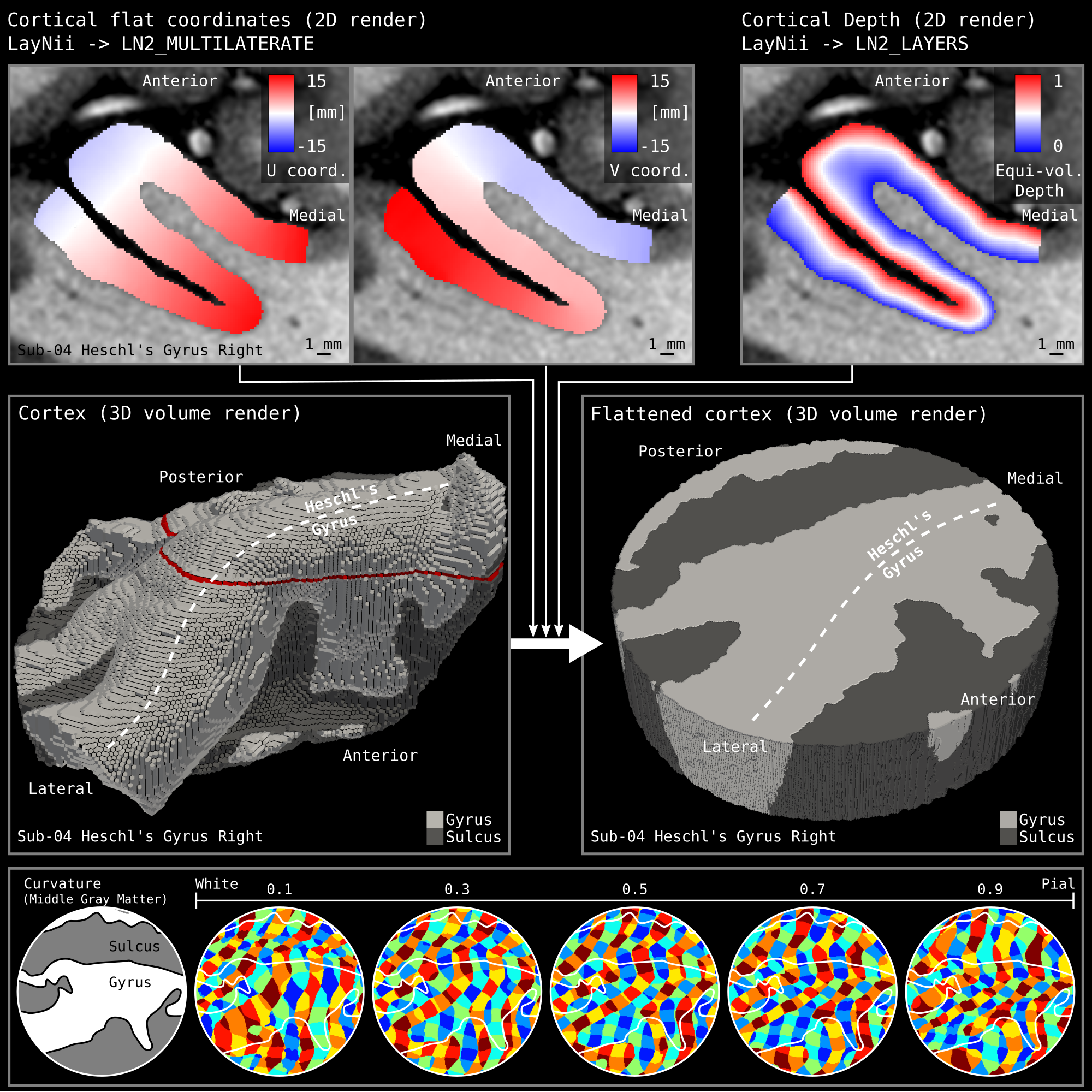
Our patch flattening method only requires one input; a segmented volume file (see Figure 1 and 2). Note that we offer a program “LN2_RIMIFY” to convert any segmented nifti file into the format preferred by LayNii.1. On the segmented volume file (referred as the ‘rim’ file in LayNii), we run our layering program “LN2_LAYERS” to measure (equi-volume) cortical depths of each voxel. We also create a middle gray matter volume. Note that, we are not using any “surfaces” (a.k.a. triangular meshes) that are commonly used in conventional MRI software. In addition, LN2_LAYERS can estimate and export cortical curvature measurements.
2. We select a single voxel that will be the center or our flattened cortex patch. For example, this voxel can be selected as the closest middle gray matter voxel to the centroid of a given activity blob. We use an interactive volume visualization and manipulation software to select this voxel (e. g. Freesurfer [1, 2], BrainVoyager [3], FSLeyes [6], ITK-SNAP [7]).
3. Using the segmented volume image together with the middle gray matter image where a center of the patch voxel is selected, our algorithm generates and parametrizes a geodesic disc around the selected voxel. Then, the developed tools find 4 points that are equally distant to each other on the perimeter of the disc (using LN2_MULTILATERATE). This step parametrizes (injects a 2D coordinate system) on the subset of the middle gray matter voxels. Then the coordinates (called UV coordinates) are propagated to the rest of the cortical thickness to cover the whole cortical depth.
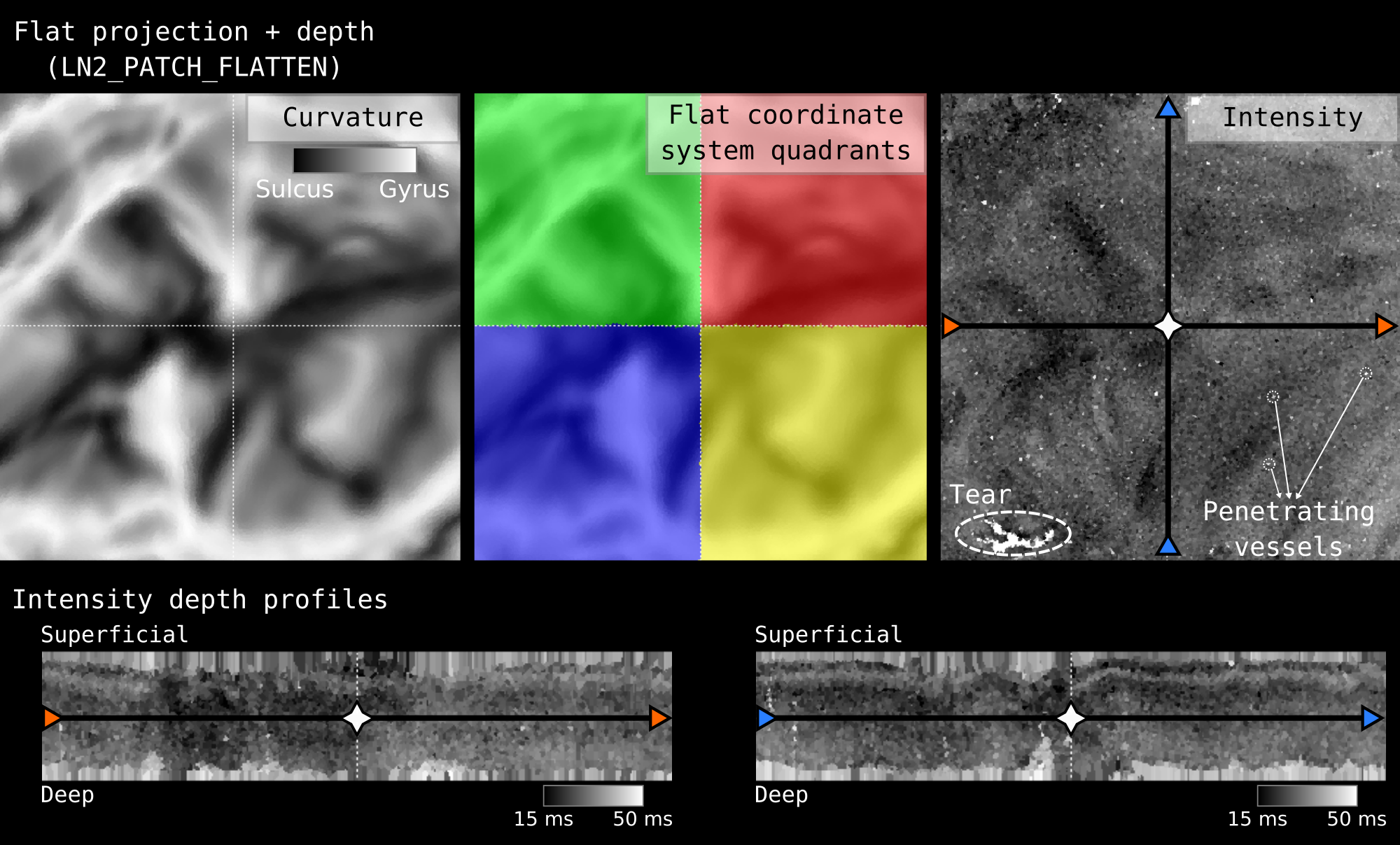
4. We use the ‘UV coordinates’ together with the equi-volume depth measurement to flatten a 3D image (e.g. T1w, or activation map) onto a new arbitrarily sized 3D rectangular lattice. This 3D flat projection with depth image is exported as a nifti file to be explored through aforementioned volume visualization softwares (see Figure 3, 4, 5).
Results & Discussion
Figure 1 and 2 demonstrate cortical patch flattening processing steps as briefly outlined above in the Methods section. It can be seen how the MRI voxel signal in the native folded brain space is seamlessly transformed into a flat Petri dish-like coordinate system. This visual representation of flat cortical patches without spatial interpolation to vertices has the ability to clearly reveal laminar and columnar structures to become visible to the naked eye, directly in the ‘raw’ MRI voxel signals.Figure 3 shows flat projections of curvature together and histology measurements from the BigBrain histological dataset. This figure exemplifies the value of the developed tools to capture subtle structural features that are not recognisable in the native cortical folded cortical space. As such, white voids of penetrating vessels become clearly visible in flattened space, while they usually disappear as single (hardly recognisable) white dots in the axial, sagittal and coronal cuts.
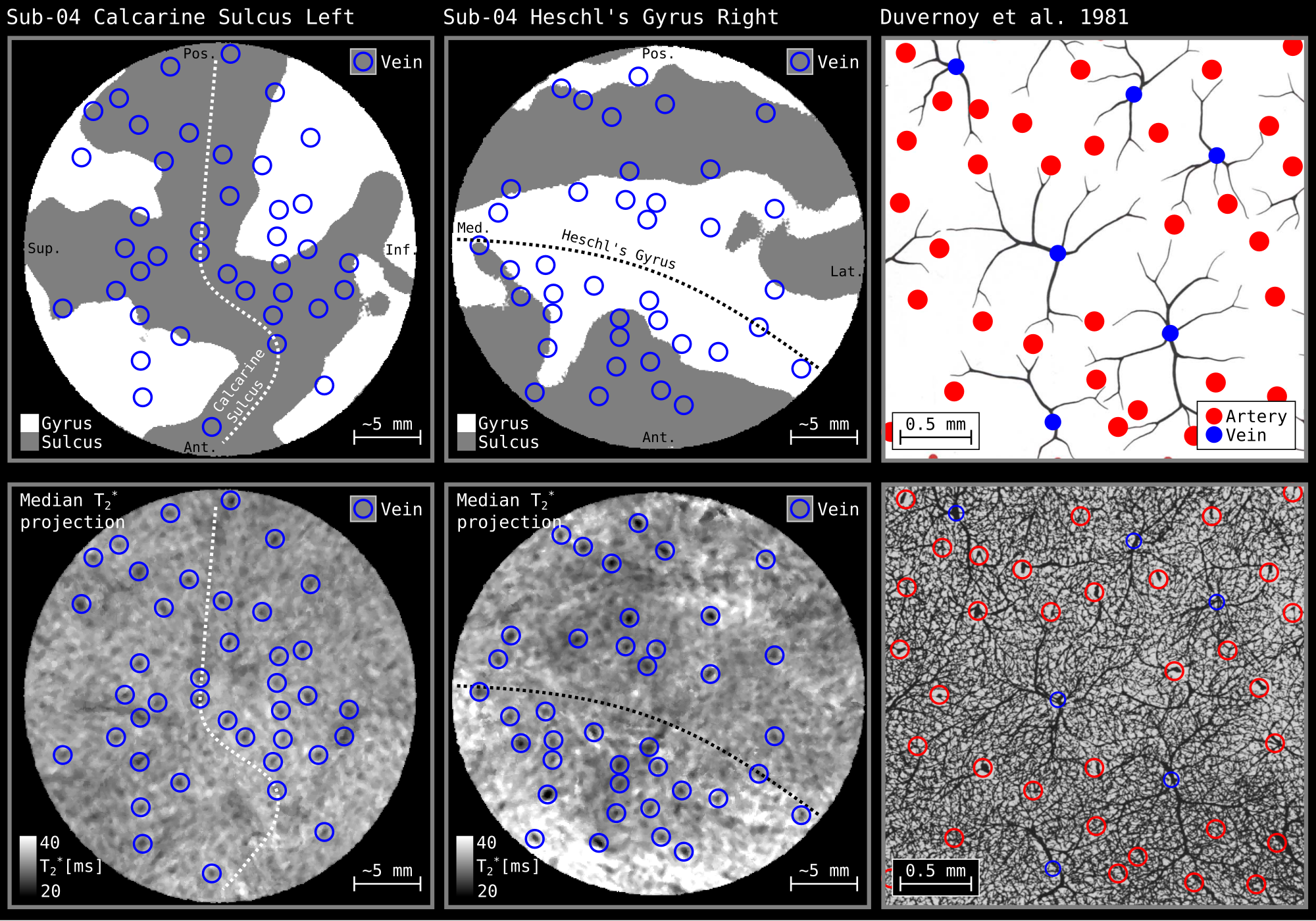
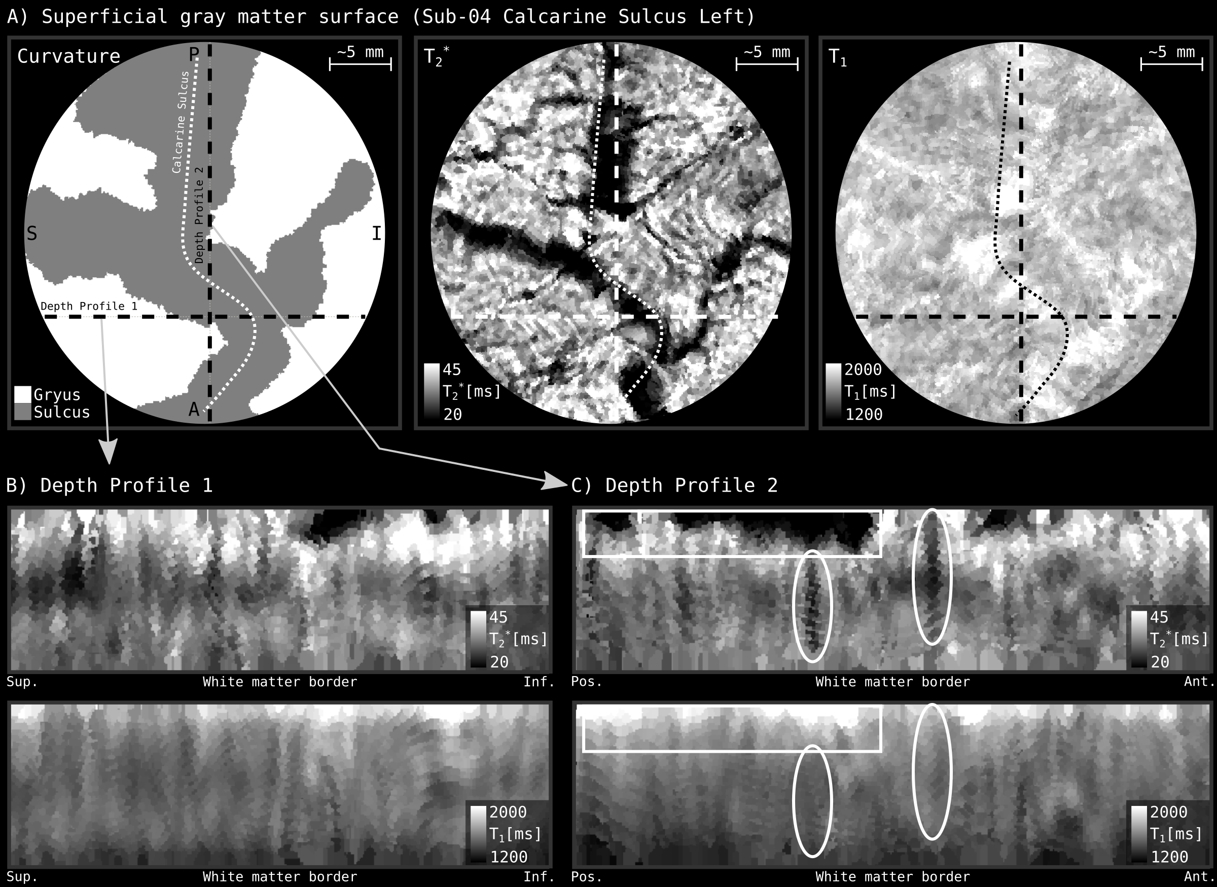
Figure 4 and 5 demonstrates our patch flattening on 0.35 mm isotropic in vivo MRI measurements (T2* and T1) [from 8] revealing cortical substructures. It can be seen that blood vessels have a dominating effect on the structural mesoscopic MRI contrast. Our tools enable topographical analysis of intra-cortical veins. Until now, this was only possible in 2D projections of cadaver brain samples [11].
Summary & Conclusion
Our new programs “LN2_MULTILATERATE” and “LN2_PATCH_FLATTEN” are able to flatten patches of cortex without requiring triangular surface meshes used in the conventional cortical flattening tools [1, 2, 3]. This is beneficial as it allows users to segment smaller volumes of cortex while offering the ability to conduct topographical surveys of the cortical landscape at very high resolutions, without the introduction of interpolation decisions until the very last visualization stage. The resulting flat patches of cortex are in Nifti format which is easy to browse with conventional volume visualization tools (fsleyes, ITKSNAP, Brainvoyager).We believe that the presented tools and their ability to reliably capture intra-cortical vessels in-vivo, will play an important role to characterize and account for vein biases in layer-dependent fMRI on a column-by-column basis. Until now such information was solely accessible in imaging animals [12].Acknowledgements
OFG and RG have financial interests tied to the company.
SB acknowledges funding from the NHMRC-NIH BRAIN Initiative Collaborative Research Grant APP1117020, NIH grant 1R01MH111419.
RH was funded by the NWO VENI project 016.Veni.198.032.
References
[1] Fischl, B., Sereno, M. I., Tootell, R. B. H., & Dale, A. M. (1999). High-resolution intersubject averaging and a coordinate system for the cortical surface. Human Brain Mapping, 8(4), 272–284. https://doi.org/10.1002/(SICI)1097-0193(1999)8:4<272::AID-HBM10>3.0.CO;2-4
[2] Fischl, B., Sereno, M. I., & Dale, A. M. (1999). Cortical surface-based analysis: II. Inflation, flattening, and a surface-based coordinate system. NeuroImage, 9(2), 195–207. https://doi.org/10.1006/nimg.1998.0396
[3] Goebel, R. (2012). BrainVoyager--past, present, future. NeuroImage, 62(2), 748–756. https://doi.org/10.1016/j.neuroimage.2012.01.083
[4] Kemper, V. G., De Martino, F., Emmerling, T. C., Yacoub, E., & Goebel, R. (2018). High resolution data analysis strategies for mesoscale human functional MRI at 7 and 9.4T. NeuroImage, 164, 48–58. https://doi.org/10.1016/j.neuroimage.2017.03.058
[5] Huber, L., ..., Gulban, O. F. (2020). LayNii: A software suite for layer-fMRI. BioRxiv. https://doi.org/10.1101/2020.06.12.148080
[6] Kay, K., Jamison, K. W., Vizioli, L., Zhang, R., Margalit, E., & Ugurbil, K. (2019). A critical assessment of data quality and venous effects in sub-millimeter fMRI. NeuroImage, 189(February), 847–869. <https://doi.org/10.1016/j.neuroimage.2019.02.006>
[7] Yushkevich, P. A., Piven, J., Hazlett, H. C., Smith, R. G., Ho, S., Gee, J. C., & Gerig, G. (2006). User-guided 3D active contour segmentation of anatomical structures: significantly improved efficiency and reliability. NeuroImage, 31(3), 1116–1128. https://doi.org/10.1016/j.neuroimage.2006.01.015
[8] Gulban, O. F. (2020). Chapter 6: In vivo T2* imaging of human auditory cortex at 350 μm isotropic resolution. Imaging the human auditory system at ultrahigh magnetic fields. ProefschriftMaken. https://doi.org/10.26481/dis.20201006og
[9] Amunts, K., Lepage, C., Borgeat, L., Mohlberg, H., Dickscheid, T., … Evans, A. C. (2013). BigBrain: An Ultrahigh-Resolution 3D Human Brain Model. Science, 340(6139), 1472–1475. https://doi.org/10.1126/science.1235381
[10] Wagstyl, K., Larocque, S., Cucurull, G., Lepage, C., Cohen, J. P. … Evans, A. C. (2020). BigBrain 3D atlas of cortical layers: Cortical and laminar thickness gradients diverge in sensory and motor cortices. PLOS Biology, 18(4), e3000678. https://doi.org/10.1371/journal.pbio.3000678
[11] Duvernoy HM. Cortical Blood Vessels of the Human Brain. Brain Res Bull. 1981;7:519-579. https://doi.org/10.1016/0361-9230(81)90007-1
[12] He Y, Wang M, Chen X, et al. Ultra-Slow Single-Vessel BOLD and CBV-Based fMRI Spatiotemporal Dynamics and Their Correlation with Neuronal Intracellular Calcium Signals. Neuron. 2018;97(4):925-939.e5. https://doi.org/10.1016/j.neuron.2018.01.025
Figures