0748
Efficient Bloch Simulation Based on Precomputed State-Transition Matrices1Institute of Medical Engineering, Graz University of Technology, Graz, Austria, 2Department of Interventional and Diagnostic Radiology, University Medical Center Göttingen, Göttingen, Germany, 3German Centre for Cardiovascular Research, Göttingen, Germany
Synopsis
The Bloch equations describe the effects of relaxation and external fields on the magnetization. Its coefficients are time-dependent, requiring computationally expensive techniques for its solution in the generic case. Currently, most techniques used in MRI are based on temporal discretization, but this requires very small time steps to achieve sufficiently small approximation errors.
In this work, we investigate a simulation technique based on a precise precomputation of state-transition matrices and compare its accuracy and efficiency with techniques based on ODE solvers and with matrix-based techniques using temporal discretization.
Introduction
While analytical solutions of the Bloch equations exist for many special cases, the solution in general needs to be determined numerically because of the time dependency of the coefficients. A conventional technique in MRI introduces temporal discretization to near a global solution based on hard-pulse and relaxation blocks leading to approximation errors. Alternatively, there exist generic methods for solving ordinary differential equations (ODE) such as Runge-Kutta solvers. They make use of higher-order approximations and can exploit adaptive step sizes to achieve a very high precision. However, these are more complex and require more computation per time step [1].In this work, we investigate a simulation technique based on state-transition matrices (STM). The state-transition matrix describes the integrated time evolution for arbitrary magnetization states for a time interval with given continuously varying external fields. Here, we use a Runge-Kutta solver with adaptive step size to precompute the state-transition matrix to a very high precision. Precomputed state-transition matrices can then be reused to efficiently simulate typical MRI sequences that are based on repetitive building blocks. We compare the accuracy and speed of the proposed method with a Runge-Kutta ODE solver and simulations based on discrete rotation matrices.
Theory
The Bloch equations are given as$$
\frac{\textrm{d}\boldsymbol{M}(t)}{\textrm{d}t}=\boldsymbol{A}(t)~\boldsymbol{M}(t)
$$
with the magnetization
$$
\boldsymbol{M}(t)=
\begin{pmatrix}
M_x(t)\\M_y(t)\\M_z(t)\\1
\end{pmatrix}
$$
and system matrix
$$
\boldsymbol{A}(t) =\begin{pmatrix}-R_2&\gamma\boldsymbol{G}_z(t)\cdot\boldsymbol{r}&-\gamma B_y(t)&0\\-\gamma\boldsymbol{G}_z(t)\cdot\boldsymbol{r}&-R_2&\gamma B_x(t)&0\\\gamma B_y(t)&-\gamma B_x(t)&-R_1&M_0R_1\\0&0&0&0\\\end{pmatrix},
$$
depending on time $$$t$$$.
The Bloch equations can be solved directly for time-dependent coefficients $$$\boldsymbol{A}(t)$$$ using Runga-Kutta methods (ODE45).
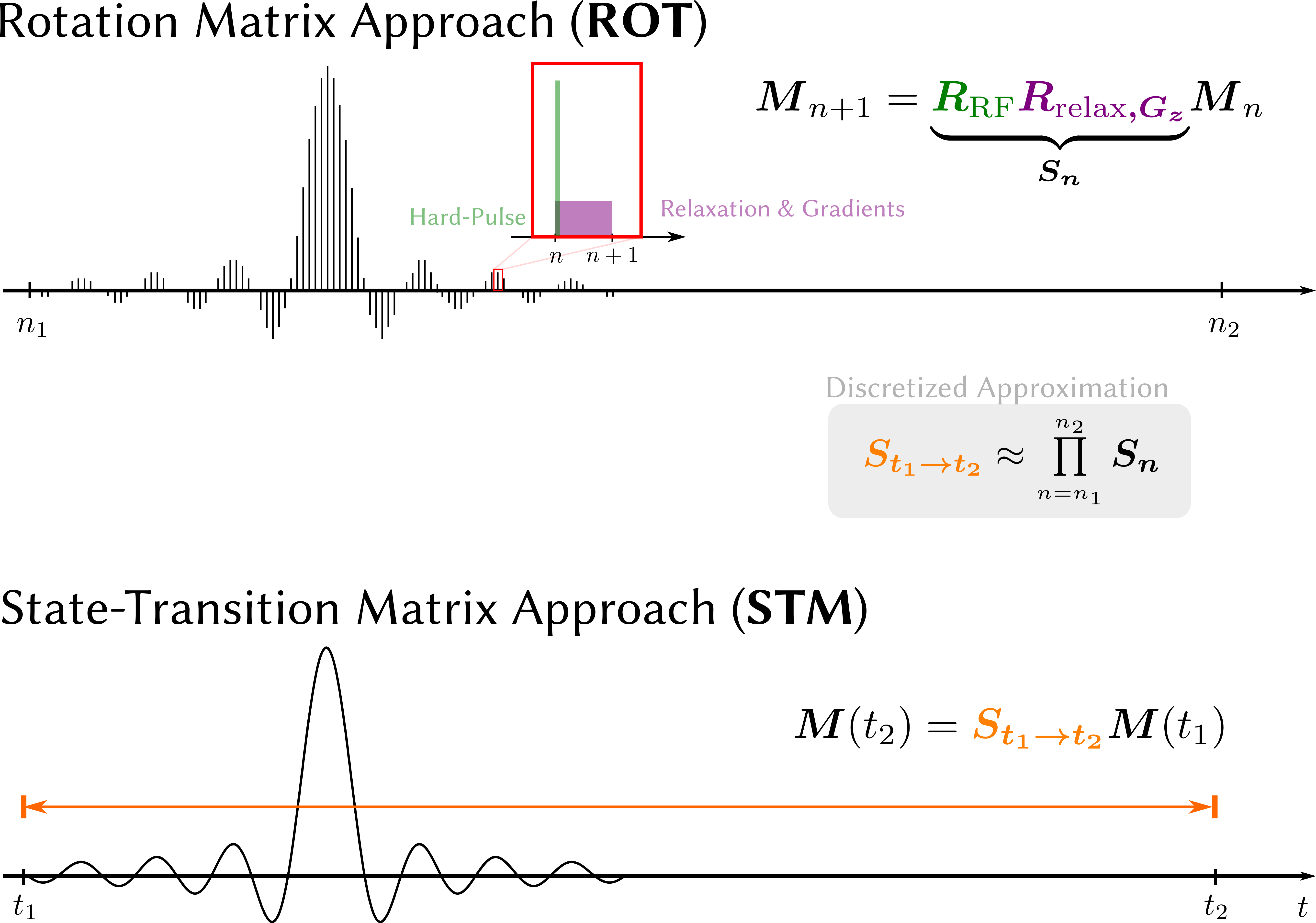
Instead of solving the Bloch equations directly, we propose the precomputation of a state-transition matrix $$$\boldsymbol{S}_{t_1\rightarrow~t_2}$$$ that describes the evolution for all magnetization states for the time from $$$t_1$$$ to $$$t_2$$$ including relaxation effects and all time dependent external RF fields (STM). Therefore, the whole temporal evolution is compressed to a multiplication with the state-transition matrix illustrated in Figure 1:
$$
\boldsymbol{M}(t_2)=\underbrace{e^{\int_{t_1}^{t_2}{\boldsymbol{A}(t)}\text{d}t}}_{\boldsymbol{S}_{t_1\rightarrow~t_2}}~\boldsymbol{M}(t_1)=\boldsymbol{S}_{t_1\rightarrow~t_2}\boldsymbol{M}(t_1).
$$
$$$\boldsymbol{S}_{t_1\rightarrow~t_2}$$$ can be approximated simply by multiplying the time-discrete matrices $$$S_n$$$ used in ROT [2].
In this work, we compute it to a very high precision. For this, we exploit that the matrix $$$\boldsymbol{S}(t):=\boldsymbol{S}_{t_1\rightarrow~t}$$$ itself fulfills an ODE given by
$$
\frac{\text{d}}{\text{dt}}\boldsymbol{S}_{t_1\rightarrow~t} = \frac{\text{d}}{\text{dt}}e^{\int_{t_1}^{t}\boldsymbol{A}(t)\text{d}t}=\boldsymbol{A}(t) e^{\int_{t_1}^{t}\boldsymbol{A}(t)\text{d}t}=\boldsymbol{A}(t)\boldsymbol{S}_{t_1\rightarrow~t},
$$
with the columns fulfilling the Bloch equations. With the initial condition $$$\boldsymbol{S}(t_1)=\boldsymbol{S}_{t_1\rightarrow~t_1}=\mathbb{1}$$$ the system can then be solved for the entries of the matrix $$$\boldsymbol{S}(t)$$$ using an ODE solver [3].
Methods
The proposed state-transition matrix technique (STM) is compared to a direct solution of the Bloch equations using the Runga-Kutta solver with adaptive step size based on weights published by Dormand and Prince (ODE54) [4]. The same solver is exploited to precompute the state-transition matrix. Additionally, a simulation technique based on temporal discretization with rotation matrices (ROT) is performed using different discretization rates of 0.1 MHz, 1 Mhz and 10 MHz. All techniques are validated in the presence of gradients and time varying external RF fields for a slice using a Hamming-windowed sinc-shaped inversion pulse with T$$$_{\text{RF}}=1$$$ ms, BWTP=1, $$$\Delta z=$$$10 mm, $$$G_z=10$$$ mT/m.The simulation speed is analyzed for a FLASH sequence with FA=8$$$^\circ$$$, TR/TE=3.1/1.7 ms and T$$$_{\text{RF}}$$$=1 ms. Relaxation parameters used in the simulations are selected to correspond to human white matter at 3T: $$$T_1/T_2=$$$832/80 ms [5].
All simulation techniques were implemented in the BART toolbox [6] using single-precision floating point arithmetic and were executed on single Intel(R) i7-8565U CPU core working at 1.80 GHz. The simulation time for estimating the temporal evolution of 100 on-resonant spins is recorded over varying numbers of repetitions.
Results and Discussion
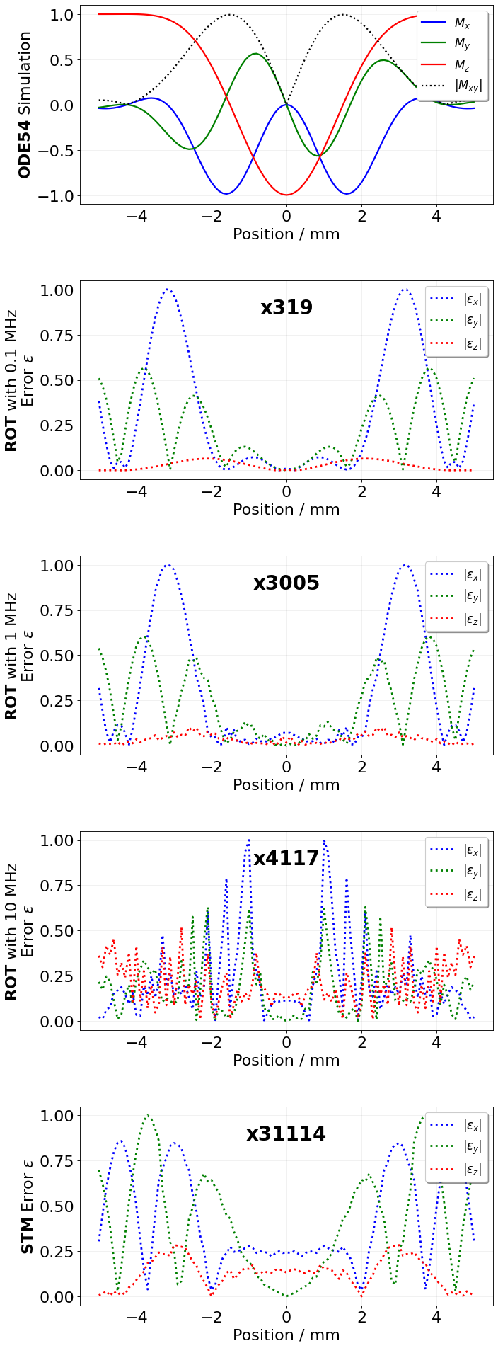
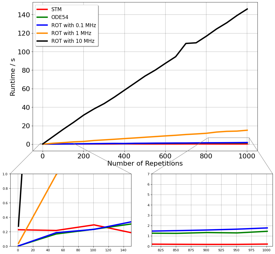
The visualization of a reference slice profile with the ODE54, the point-wise deviation to the ODE54 simulation of ROT at different rates and the STM simulation are shown in Figure 2. As expected, the differences of ROT decrease with increasing sampling rate. The highest sampling rate is already affected by numerical noise due to limited floating point precision. With the parameters used here for the computation of the state-transition matrix, the STM technique has substantially lower error than all versions of ROT.The simulation times are shown in Figure 3. The constant offset of the STM simulation is higher compared to the other techniques which reflects the initial calculation of the state-transition matrix. The other methods are therefore faster for a small number of repetitions. Nevertheless, this changes markedly for more repetitions because the STM technique only requires a single matrix multiplication per TR, while the ODE54 and the ROT require more time to simulate each additional TR. The computational costs of ROT also increase substantially for higher rates.
While the slice-profile analysis confirms the high accuracy of the STM technique, the computation time analysis demonstrates substantial efficiency gains compared to alternative methods for sequences with many repetitions.
Conclusion
This work explores the use of state-transition matrices precomputed with a high precision using an adaptive step size Runge-Kutta solver for fast and accurate simulation of complex spin dynamics. By modelling the time-dependent spin evolution with a single matrix, it reduces the computational costs for sequences with many similar repetitions. The technique is compared with respect to accuracy and speed to a Runge-Kutta simulation and approaches based on temporal discretization with rotation matrices.Acknowledgements
No acknowledgement found.References
[1] C. Graf, et al. Accuracy and performance analysis for Bloch and Bloch-McConnell simulation methods. J. Magn. Reson. 329 (2021).
[2] S.J. Malik, et al. Steady-state imaging with inhomogeneous magnetization transfer contrast using multiband radiofrequency pulses. Magn. Reson. Med. 83 (2020).
[3] C. Moler, C. van Loan. Nineteen Dubious Ways to Compute the Exponential of a Matrix, Twenty-Five Years Later*. SIAM Review 45 (2003).
[4] J.R. Dormand, P.J. Prince. A family of embedded Runge-Kutta formulae. J. Comput. Appl. Math. 6 (1980).
[5] J.P. Wansapura, et al. NMR relaxation times in the human brain at 3.0 tesla. J. Magn. Reson. Imag. 9 (1999).
[6] M. Uecker, et al. Software Toolbox and Programming Library for Compressed Sensing and Parallel Imaging. ISMRM Workshop on Data Sampling and Image Reconstruction, Sedona 2013.
Figures