1227
3D-Simulation of Flowing Spins using the Lattice Boltzmann Method with Maxwell Diffuse Reflection Boundaries1Insitut of Medical Engineering Graz, Graz, Austria, 2Institut Diagnostic and Interventional Radiologie, Göttingen, Germany, 3Max Planck Institute for Dynamics and Self-Organization, Göttingen, Germany, 4Institut of Medical Engineering, Graz, Austria
Synopsis
The lattice Boltzmann method (LBM) is a powerful technique to simulate complex fluid dynamical systems. The extension of the LBM to flow with a spin degree of freedom in external magnetic fields has shown promising results in 2D. Here, we describe first 3D numerical results utilizing extended kinetic-theory based boundary conditions. The simulation of a laminar pipe flow is verified on the Pouiseuille flow and shown to be able to predict signal changes caused by in-flow effects as expected from previous flow experiments.
Synopsis
The lattice Boltzmann method (LBM) is a powerful technique to simulate complex fluid dynamical systems. The extension of the LBM to flow with a spin degree of freedom in external magnetic fields has shown promising results in 2D. Here, we describe first 3D numerical results utilizing extended kinetic-theory based boundary conditions. The simulation of a laminar pipe flow is verified on the Pouiseuille flow and shown to be able to predict signal changes caused by in-flow effects as expected from previous flow experiments.Introduction and Purpose
Fluid dynamics and corresponding imaging artifacts of flow in MRI are not fully understood. Simulations can be utilized to investigate these effects. In contrast to previous numerical techniques1, the lattice Boltzmann method (LBM)2 allows modelling of fully coupled flow and diffusion dynamics. Previously, we extended a two dimensional LBM with a joint velocity-spin distribution and recovered the Navier-Stokes equations and Bloch-Torrey equations, as well as, predicted results of a MR flow experiment3. Conventional boundary conditions do not probably describe the redistribution of spins reflecting at a wall. Here, we therefore extend Maxwell Diffuse Reflection Boundaries4, which are based on kinetic-theory, to velocity-spin distribution. Furthermore, we compare the predicted in-flow effect in a 3D laminar pipe flow with experimental results3.Theory
A model of flowing particles with spin 1/2 using a matrix-valued semi-classical velocity-spin distribution $$$D(\vec r, t)$$$ as an extension of the conventional LBM velocity distribution $$$f(\vec{r}, \vec{u}, t)$$$ was proposed previously3. Here $$$\vec{r}$$$ is the location on a spatial grid, $$$\vec{c}$$$ the velocity and $$$t$$$ the time step. Using the expansion of a quantum mechanical density operator $$$D$$$ of 1/2 particles into Pauli matrices, the velocity-spin distribution $$$D(\vec r, \vec{u}, t)$$$ is discretized by:$$D_i(\vec r, t) := \frac{1}{2} \sum_j f_{i,j}(\vec r, t) \sigma_j, $$
where $$$i$$$ is an index of the discretized velocity direction $$$\vec{c}_i$$$, $$$j$$$ denotes the polarization direction {$$$0,x,y,z$$$}, and $$$\sigma_j$$$ is the corresponding Pauli matrix, with $$$\sigma_0$$$ the identity matrix. The macroscopic magnetization $$$\vec{M}$$$, density $$$\rho$$$ and velocity $$$\vec{u}$$$, are equal to the expectation values of the distribution:
$$\rho = \sum_i f_{i,0}, \qquad \rho \vec u = \sum_i f_{i,0} \vec c_i, \quad \text{ and } \quad M_j = \sum_i f_{i,j} \text{ .}$$
In the LBM, streaming and collision steps are used to simulate the discretized Boltzmann equation2. The streaming step transports $$$f_{i,j}$$$ to the next grid point in the direction $$$\vec c_i$$$. The collision step locally relaxes $$$f_{i,j}$$$ towards a equilibrium distribution $$$f^{eq}_{i,j}(\rho, \vec{u})$$$. An additional matrix multipication during the collision step changes $$$f_{i,j}$$$ according to the time-discretized Bloch equations2.
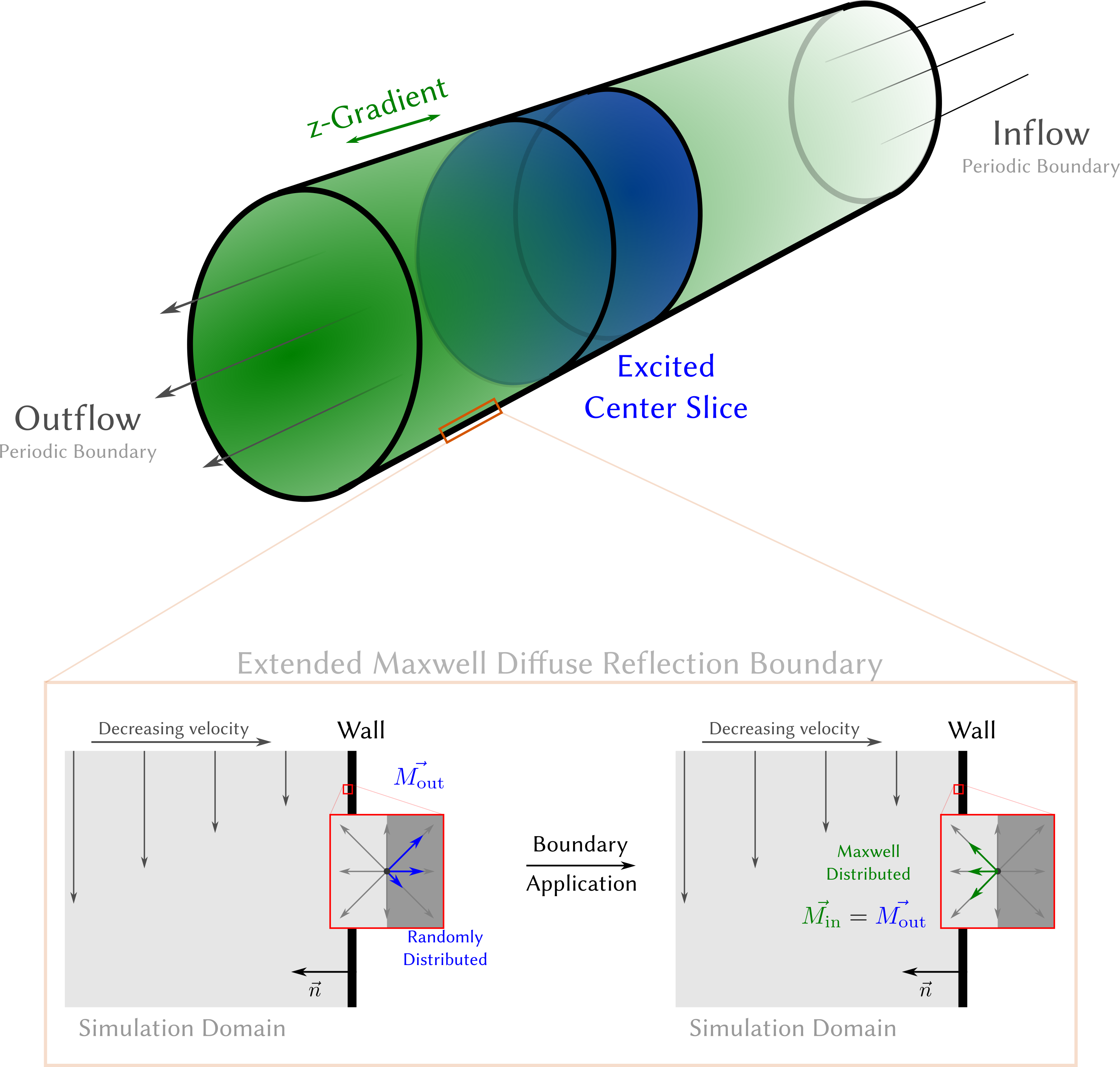
Here, the model is extended to 3D using a D3Q27 lattice. The kinetic-theory based boundary approach is used (see Figure 1) to determine the unknown inflowing distributions from the known outflowing distributions after the streaming step4. The mean velocity at the wall is zero, thus the particle motion driven by diffusion and independent of its inital state, with small deviation from the equilibrium distribution $$$f^{eq}_{i,j}(\rho, \vec{u})$$$. At equilibrium all elementary processes are equal to their reverse, hence the inflowing distributions are also Maxwell-Boltzmann distributed. By weighting the inflowing Maxwell-Boltzmann distribution by the outflowing magnetization and density to ensure their conservation we obtain the Maxwell Diffuse Reflection Boundary extended to spin-velocity distribution.
Methods
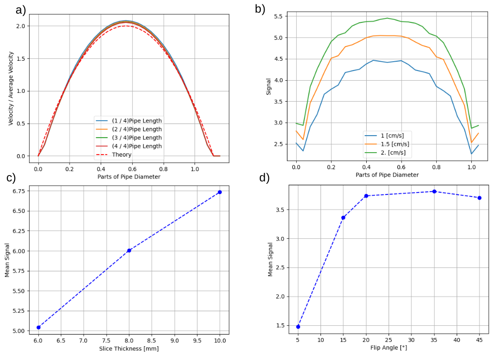
Utilizing the setup shown in Figure 1, a laminar pipe flow was considered and compared to the expected Pouiseuille flow. An aspect ratio (length/diameter) of a third and a Reynolds number (Re) of 100 were used.To validate the signal change caused by in-flow effects, a spoiled phase-contrast FLASH sequence (TR = 11ms, TE = 9.47ms) was applied with the excited slice located in the middle of the pipe. The slice profile is simulated by a slice-selective pulse and a gradient. The velocities, slice thickness and flip angle were varied. The signal intensities were compared to previous experimental results reported in 3.
The simulation using a [31/31/91] grid was run in parallel on a AMD Ryzen 7 5800-x prozessor with 8 kernel.
Results
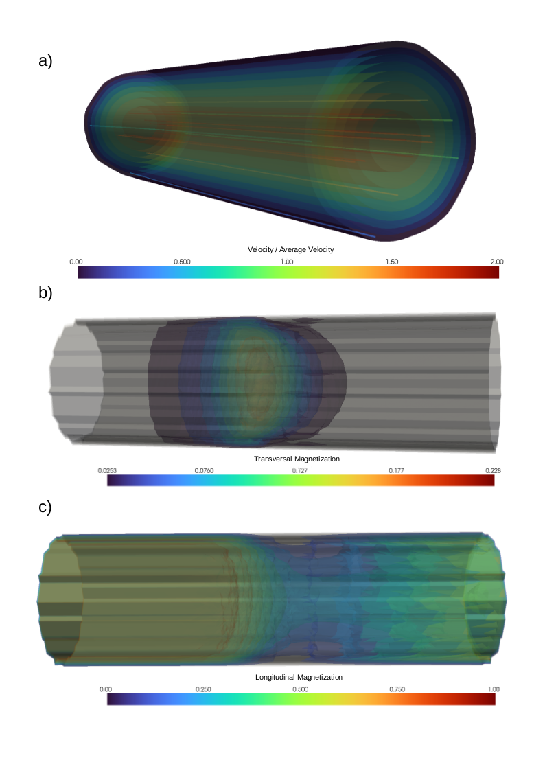
Figure 2 shows the predicted streamlines and contours for the velocity and magnetization. As expected, the velocity streamlines are straight lines and the contours are round circles with decreasing radius, proving that the profile is consistent through the pipe. The transversal magnetization shows parabolic contour lines in flow direction after the excited slice, and straight ones in the opposite direction: The flow drags the inverted magnetization forward in flow direction. In contrast, at the boundaries, the profile is more symmetric and the maximal longitudinal magnetization (0.059) is close to the steady-state value (0.057).Figure 3 shows the comparison of the theoretically and numerically obtained cross-sectional flow profiles, as well as, the signal for varying flow rates, slice thickness and flip angle.
Discussion and Outlook
We extended a method for simulating combined spin and fluid physics to 3D. We further integrated kinetic-based boundaries and simulated the slice-selection pulse. For the in-flow effect, the numerical results correspond well to previously reported experimental results. Due to the simulation times of 10h a coarse discretization has to be used limiting the simulation to laminar flow and to a low accuracy. A parallel GPU implementation and improved methods for the magnetization based on precomputed state-transition matrices5 are suggested.Acknowledgements
No acknowledgement found.References
[1] Jurczuk K., Kretowski M., Bellanger J., Eliat P., Saint-Jalmes H., Bézy-Wendling J. (2013) Computational modeling of MR flow imaging by the lattice Boltzmann method and Bloch equation. In Mag. Res. Imag. Vol 31; 7.
[2] Krüger T., Halim K. (2017) The Lattice Boltzmann Method, Springer-Verlag.
[3] Adler A., Kollmeier JM., Scholand N., Rosenzweig S., Wang Y., Uecker M. (2021) Simulation of Flowing Spins in MRI using the Lattice Boltzmann Method. ISMRM 2021. Proc. Intl. Soc. Mag. Reson. Med. 29; 2100.
[4] Ansumali, Santosh & Karlin, Iliya. (2002) Kinetic boundary conditions in the lattice Boltzmann method. Physical review. E, Statistical, nonlinear, and soft matter physics. 66. 026311. 10.1103/PhysRevE.66.026311.
[5] Scholand N., Graf C., Uecker M. (2022) Efficient Bloch Simulation Based on Precomputed State-Transition Matrices. Submitted to ISMRM 2022.
Figures