1700
Sensitivity Analysis of the Bloch Equations1Institute of Medical Engineering, Graz University of Technology, Graz, Austria, 2Department of Interventional and Diagnostic Radiology, University Medical Center Göttingen, Göttingen, Germany, 3German Centre for Cardiovascular Research, Göttingen, Germany
Synopsis
Algorithms for pulse optimization, quantitative MRI, or model-based reconstruction require knowledge about partial derivatives of the Bloch equations.While being available for specific analytical solutions, computing them becomes challenging in the general case. Difference quotient techniques can be used, but require perturbation tuning to avoid errors.
In this work, we investigate the use of direct sensitivity analysis to estimate the partial derivatives of the Bloch equations. We validate it with an analytical sequence model and compare it to the difference quotient in an example without analytical solution. In all cases, direct sensitivity analysis provided highly accurate estimates of the partial derivatives.
Introduction
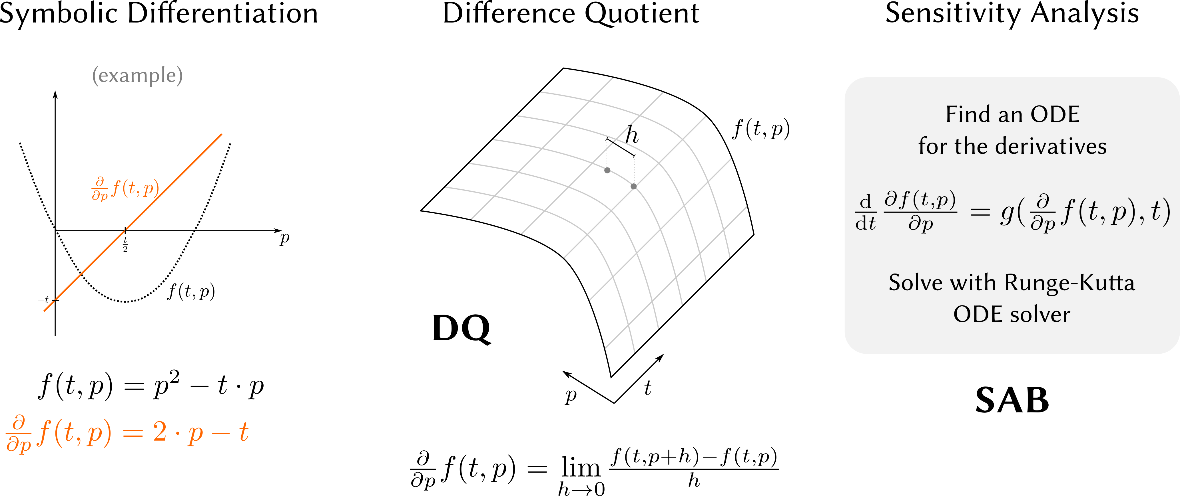
Estimating partial derivatives of the Bloch equations can be performed numerically using the difference quotient, but this requires careful tuning of the perturbation $$$h$$$ for each optimized parameter or an automatic adaptive strategy that may require repeated computation of solutions of the Bloch equations.In this work, we investigate the application of direct sensitivity analysis to the Bloch equations (SAB). We derive an ordinary differential equation (ODE) that describes the temporal evolution of the partial derivatives and solve it with a Runge-Kutta solver.
We validate the accuracy of the estimated partial derivatives for the relaxation parameters $$$R_1$$$, $$$R_2$$$ and the radio-frequency (RF) $$$B_1$$$ by comparison with an analytical model for an Inversion-Recovery balanced SSFP (IR-bSSFP) sequence. Additionally, we compare them to the derivatives of a non-analytical solution for the IR-bSSFP sequence without leading $$$\alpha/2$$$ pulse obtained by computing the difference quotients.
Theory
We consider an ODE system that describes the temporal evolution of a vector $$$\boldsymbol{y}(\boldsymbol{c},t)$$$ depending on a vector of parameters $$$\boldsymbol{c}$$$ and the time $$$t$$$. Each element $$$y_i(\boldsymbol{c},t)$$$ follows$$
\frac{\text{d}}{\text{dt}}y_i(\boldsymbol{c},t)=f_i(\boldsymbol{y}(\boldsymbol{c},t),t,\boldsymbol{c}).
$$
The $$$(i,j)$$$-th entry of the sensitivity matrix $$$\boldsymbol{Z}(t)$$$ with respect to the parameter $$$\boldsymbol{c}_j$$$ is defined as
$$
Z_{ij}(t)=\frac{\partial{y_i(\boldsymbol{c},t)}}{\partial{{c}_j}}.
$$
The direct sensitivity analysis [1] estimates the entries of $$$\boldsymbol{Z}(t)$$$ by defining a set of differential equations that describe the temporal behavior of $$$\frac{\text{d}\boldsymbol{Z}(t)}{\text{d}t}$$$.
Assuming that the partial and ordinary derivatives interchange, the $$$(i,j)$$$-th entry of $$$\boldsymbol{Z}$$$ follows
$$
\frac{\text{d}}{\text{d}t}Z_{ij}(t)=\frac{\text{d}}{\text{d}t}\left(\frac{\partial{y_i}(\boldsymbol{c},t)}{\partial{{c}_j}}\right)=\frac{\partial}{\partial{{c}_j}}\left(\frac{\text{d}{y_i}(\boldsymbol{c},t)}{\text{d}t}\right).
$$
Substituting $$$\frac{\text{d}{y_i}(\boldsymbol{c},t)}{\text{d}{t}}$$$ yields
$$
\frac{\text{d}}{\text{d}t}Z_{ij}(t)=\frac{\partial}{\partial{\boldsymbol{c}_j}}f_i(\boldsymbol{y}(\boldsymbol{c},t),t,\boldsymbol{\boldsymbol{c}}).
$$
With the chain rule, the resulting ODE becomes
$$
\frac{\text{d}}{\text{d}t}Z_{ij}(t)=\frac{\partial{f_i}(\boldsymbol{y}(\boldsymbol{c},t),t,\boldsymbol{\boldsymbol{c}})}{\partial{\boldsymbol{c}_j}}+\sum\limits_{j}\frac{\partial{f_i}(\boldsymbol{y}(\boldsymbol{c},t),t,\boldsymbol{\boldsymbol{c}})}{\partial{y_j}}\frac{\partial{y_j}(\boldsymbol{c},t)}{\partial{\boldsymbol{c}_j}}=\frac{\partial{f_i}(\boldsymbol{y}(\boldsymbol{c},t),t,\boldsymbol{\boldsymbol{c}})}{\partial{\boldsymbol{c}_j}}+\sum\limits_{j}\frac{\partial{f_i}(\boldsymbol{y}(\boldsymbol{c},t),t,\boldsymbol{\boldsymbol{c}})}{\partial{y_j}}Z_{ij},
$$
where $$$\frac{\partial{f_i}(\boldsymbol{y}(\boldsymbol{c},t),t,\boldsymbol{\boldsymbol{c}})}{\partial{y_j}}$$$ describes the $$$(i,j)$$$-th element of the Jacobian $$$J_{i,j}$$$. This can be written compactly for the complete sensitivity matrix as
$$
\frac{\text{d}}{\text{d}t}\boldsymbol{Z}(t)=\boldsymbol{f_c}(\boldsymbol{y}(\boldsymbol{c},t),t,\boldsymbol{\boldsymbol{c}})+\boldsymbol{J}(\boldsymbol{y}(\boldsymbol{c},t),t,\boldsymbol{\boldsymbol{c}})\cdot\boldsymbol{Z}(t).
$$
If direct sensitivity analysis is applied to the Bloch equations for the parameters $$$R_1$$$, $$$R_2$$$ and $$$B_1$$$, the ODE of the sensitivities becomes
$$
\frac{\text{d}}{\text{d}t}\boldsymbol{Z}=\begin{pmatrix}0&-M_x&-\gamma\sin\phi~\omega_1M_z\\0&-M_y&\gamma\cos\phi~\omega_1M_z\\M_0-M_z&0&\gamma(\sin\phi~\omega_1M_x-\cos\phi~\omega_1M_y)\end{pmatrix}~~~~+\begin{pmatrix}-R_2&\gamma{B_z}&-\gamma\sin\phi~\omega_1B_1\\-\gamma{B_z}&-R_2&\gamma\cos\phi~\omega_1B_1\\\gamma\sin\phi\omega_1B_1&-\gamma\cos\phi~\omega_1B_1&-R_1\end{pmatrix}\cdot\boldsymbol{Z}.
$$
Afterwards, the ODE need to be solved simultaneously with the Bloch equation ODE to estimate the time dependent parameters $$$M_x$$$, $$$M_y$$$ and $$$M_z$$$ necessary for the calculation of the sensitivity matrix $$$\boldsymbol{Z}$$$.
Methods
The partial derivatives with respect to the parameters $$$R_1$$$, $$$R_2$$$ and $$$B_1$$$ are calculated for an IR-bSSFP sequence assuming heart septal tissue with $$$T_1/T_2=$$$ 1250/45 ms [2]. The ODE derived with direct sensitivity analysis is solved using a Runge-Kutta algorithm with adaptive step size using weights published by Dormand and Prince (DOPRI54) [3], defining the proposed SAB technique.For comparison, two simulations are performed for each parameter differing by a small perturbation $$$h$$$, which allows us to estimate the derivatives by computing the difference quotients DQ. Both techniques are compared to the symbolic derivatives of the well known analytical solution of the Bloch equations for the IR-bSSFP sequence [4].
Additionally, the partial derivatives with respect to the parameters of a non-analytical solution of the IR-bSSFP model without leading $$$\alpha/2$$$ pulse are computed using SAB and DQ and compared.
All techniques were implemented in the BART toolbox [5] using single-precision floating point arithmetic.
Results and Discussion
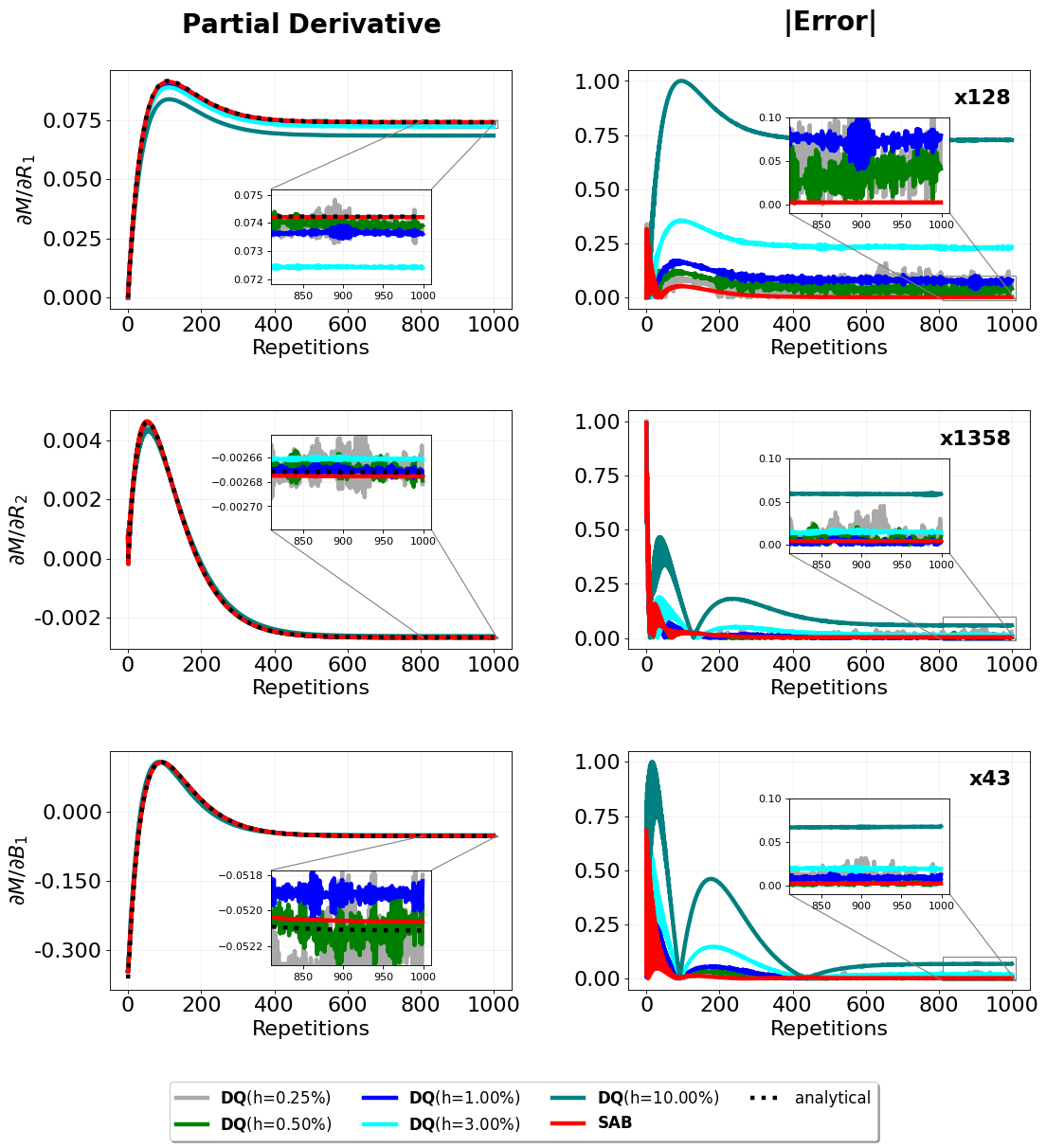
The partial derivatives for the IR bSSFP sequence and the errors of the SAB method and the DQ method for various perturbations $$$h$$$ are shown in Figure 2. As expected, the error of DQ decreased for small perturbations until numerical noise started to dominate for very small $$$h$$$.The developed SAB performed best in all cases. While DQ with $$$h=1\%$$$ perturbation from the original parameter led to equally good results in the $$$R_2$$$ derivative, its error was high for $$$R_1$$$ and $$$B_1$$$, emphasizing the need of tuning the perturbation level in DQ methods.
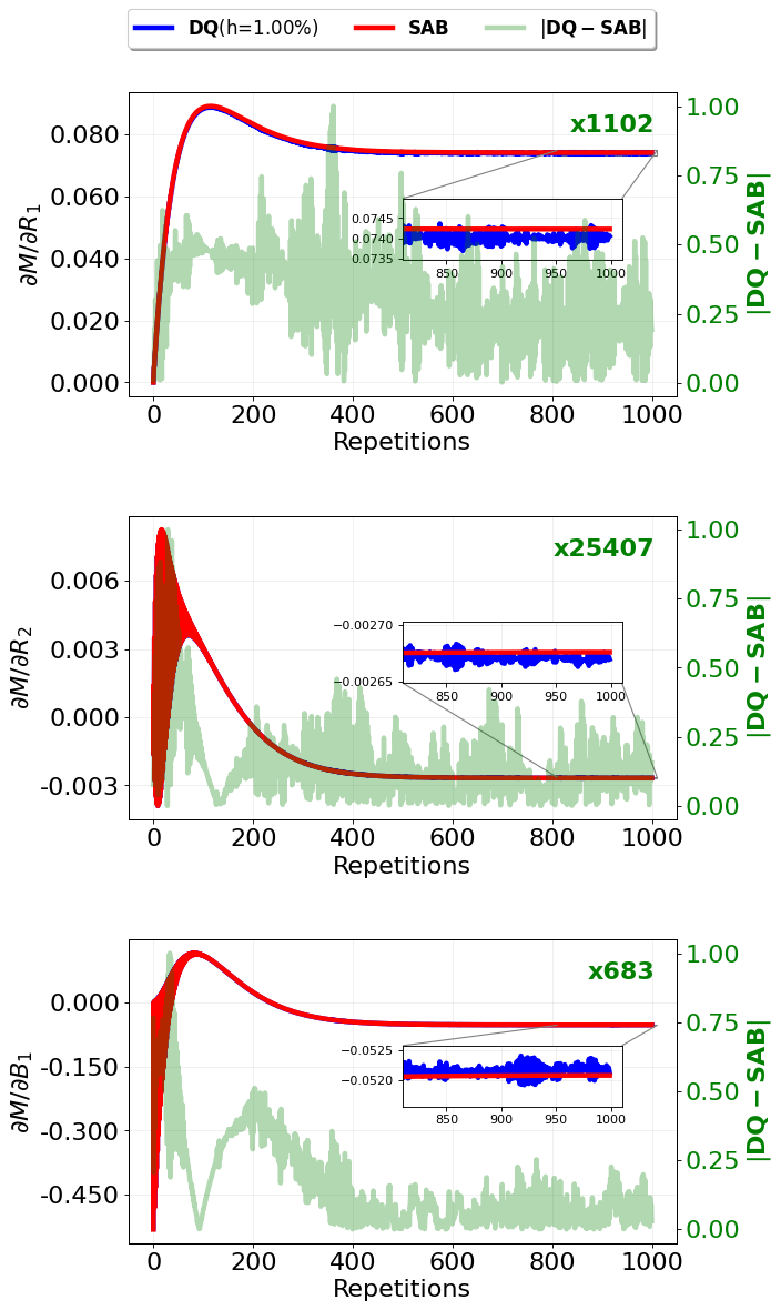
The derivatives estimated for the non-analytical signal for the IR-bSSFP without $$$\alpha/2$$$ pulse are shown in Figure 3.The differences between SAB and DQ with manually chosen $$$h=1\%$$$ are very small. Following the zoom-in in Figure 3, the observable noise in the green difference line results from numerical noise amplification for the chosen perturbation in the DQ method.
The analytical IR bSSFP and non-analytical model analysis confirm the high accuracy of the SAB technique for generic signal models without the need for parameter tuning and with low numerical noise.
Conclusion
This work explored the application of direct sensitivity analysis to the Bloch equations. By solving the resulting ODE for the sensitivity matrix with a Runge-Kutta solver, a simple technique is obtained that is capable of calculating precise and numerically stable partial derivatives for generic non-analytical solutions.The technique is validated by comparison with the symbolic derivatives for an analytical solution for the IR-bSSFP sequence and compared to the difference quotient with varying perturbation size. We also show a comparison with the difference quotient for an example where no analytical solution is known.
Acknowledgements
No acknowledgement found.References
[1] R.P. Dickinson and R.J. Gelinas. Sensitivity analysis of ordinary differential equation systems - A direct method. J. Comp. Phy. 21(2) (1976).
[2] P. Kellman and M.S. Hansen. T1-mapping in the heart: accuracy and precision. J. Cardio. Magn. Reson. 16 (2014).
[3] J.R. Dormand and P.J. Prince. A family of embedded Runge-Kutta formulae. J. Comput. Appl. Math. 6(1) (1980).
[4] P. Schmitt, et al. Inversion recovery TrueFISP: Quantification of T1, T2, and spin density. Magn. Reson. Med. 51 (2004).
[5] M. Uecker, et al. Software Toolbox and Programming Library for Compressed Sensing and Parallel Imaging. ISMRM Workshop on Data Sampling and Image Reconstruction, Sedona 2013.
Figures